Function
A function takes in some input and evaluates an output. You may be familiar with function notation like this: \[S(x) = \sqrt{x}\] which defines a function \(S\) that takes an input \(x\) and evaluates the output as the square-root of \(x\). For example, \[ S(64) = 8 \] \[ S(5929) = 77 \] \[ S(42) \approx 6.48074 \] For real numbers, the domain of \(S(x)\) is all valid inputs \(x \geq 0\), and the codomain is all possible outputs \(y \geq 0\).
Feedback
It can be useful to represent the process of evaluating a function \(F(x)\) with a block diagram:
Feedback is a procedure where the output of a process is fed back into the input. Each time this happens is one iteration. Starting with some initial condition \(x_{0}\), we iterate the function on \(x_{0}\) to get the output \(x_1\), then iterate to get \(x_2\), etc.

Let's use our square root function from above as an example, and choose an initial value of \(x_0 =16\). We can iterate once to get \(S(16)=4\), then take that output and put it back into \(S(x)\) to get: \[S(S(16)) = \sqrt{\sqrt{16}} = 2 \text{.}\]
Given an initial condition \(x_0\), then we would have: \[x_1 = S(x_0)\] \[x_2 = S(x_1) = S(S(x_0))\] \[x_3 = S(x_2) = S(S(S(x_0)))\] \[x_n = S(x_{n-1}) = S^{n}(x_0) \]
We use a superscript notation \(x_n = F^{n}(x_0)\) to represent \(n\) iterations in \(F\) on an initial value \(x_0\text{.}\) We view these functions as dynamical systems since they have state and evolve over time.
This process of feedback, where the state of a system at the next step is dependent on the current state of the system, is fundamental to dynamical systems and arises across domains. Many data pipelines that feed into models are components of dynamical systems with feedback, as the output of those models often will influence the next generation of inputs.
Consider a movie recommendation system on a streaming service. One input that such a system is likely to include is the set of movies a user has already watched. These are a factor in determining recommendations for other movies to watch. The user may or may not watch those recommended movies which changes the input for the next recommendation.
A real system can be far more complex. Other examples of feedback systems include:
- Home thermostat
- A car's cruise control
- Population growth
- A video camera being show its own video feed
- Technological advancement
- College rankings
Orbit
Given an initial value \(x_0\), iterating in a function \(F(x)\) generates a sequence of outputs we call the orbit of \(x_0\). Consider the dynamical system: \[F(x) = x^2 - \sin(x) \] Below are the first 20 values in the orbits of \(x_0 = -0.1, 0.23, 1, 1.5,\) and \(2\text{.}\)
| n | \(x_0 = -0.1\) | \(x_0=0.23\) | \(x_0=1\) | \(x_0=1.5\) | \(x_0=2\) |
| 1 | 0.1098334166 | -0.1750775235 | 0.1585290152 | 1.252505013 | 3.090702573 |
| 2 | -0.09754934336 | 0.2048366158 | -0.1327343898 | 0.6189972808 | 9.501574278 |
| 3 | 0.1069105801 | -0.1614491549 | 0.1499633895 | -0.1970611434 | 90.35663462 |
| 4 | -0.09527716197 | 0.1868145137 | -0.1269129148 | 0.2346212961 | 8163.640109 |
| 5 | 0.1042108148 | -0.1508301185 | 0.1426793817 | -0.1774275213 | 66645018.85 |
| 6 | -0.09316240354 | 0.1730086027 | -0.1218383712 | 0.2079785922 | 4.44156E+15 |
| 7 | 0.1017069324 | -0.1422148353 | 0.1363817435 | -0.1632273811 | 1.97274E+31 |
| 8 | -0.09118737513 | 0.1619609953 | -0.1173593736 | 0.189146708 | 3.89172E+62 |
| 9 | 0.09937619245 | -0.1350224831 | 0.1308633788 | -0.1522444128 | 1.51455E+125 |
| 10 | -0.08933707853 | 0.1528436605 | -0.1133649638 | 0.174835326 | 2.29386E+250 |
| 11 | 0.09719940465 | -0.1288880692 | 0.1259739144 | -0.1433785851 | Explodes... |
| 12 | -0.08759870047 | 0.1451436488 | -0.1097715626 | 0.1634452596 | |
| 13 | 0.09516024386 | -0.1235678908 | 0.1216010371 | -0.1360041557 | |
| 14 | -0.08596121671 | 0.1385226942 | -0.1065147644 | 0.1540823926 | |
| 15 | 0.09324472062 | -0.1188915743 | 0.117658865 | -0.129732044 | |
| 16 | -0.08441508084 | 0.1327468858 | -0.1035439738 | 0.1461988463 | |
| 17 | 0.09144076678 | -0.1147356217 | 0.1140804055 | -0.1243044884 | |
| 18 | -0.0829519772 | 0.1276483153 | -0.1008187807 | 0.1394362241 | |
| 19 | 0.08973790793 | -0.1110078529 | 0.1108124999 | -0.119542372 | |
| 20 | -0.08156462268 | 0.1231027499 | -0.0983064436 | 0.1335482365 |
Spreadsheets are excellent tools for exploring systems like this.
Types of Orbits
There are many interesting types of orbits in dynamical systems. We will take a closer look at:
- Convergent
- Divergent
- Constant (fixed point)
- Periodic (cyclic)
- Chaotic
Convergent and Divergent Orbits
An orbit converges if it approaches a constant \(c\), i.e., \[ \lim_{n \to \infty} x_n = c \] Our square root system, \(S(x)=\sqrt{x}\), converges toward \(1\) for all positive values.
An orbit diverges if it does not converge, but we are especially interested in divergent orbits when they go off toward \(\pm \infty \text{.}\) Consider the doubling system, \(D(x)=2x\). The orbit of any positive value \(x_0\) will go toward \(\infty\) under \(D(x)\), while the orbit of any negative \(x_0\) goes toward \(-\infty\text{.}\)
Fixed Point
A fixed point in a dynamical system \(F(x)\) is a value \(x^{*}\) such that \[F(x^{*}) = x^{*}\] \(S(x)=\sqrt{x}\) has two fixed points: \(x^{*}=0\) and \(x^{*}=1\).
Finding fixed points may involve analytical, numerical, or graphical solutions. Graphically, finding a point on \(F\) such that \(F(x)=x\) is equivalent to finding an intersection between \(F(x)\) and \(y=x\).

Periodic Orbit
A periodic orbit is an orbit which contains a cycle, or repeating sequence of values. A fixed point is really a \(1\)-cycle periodic orbit! An example of a \(2\)-cycle is the orbit of \(x_0=3\) under \(A(x)=-x\), which we find to be: \(3,-3,3,-3,...\text{.}\)
A \(2\)-cycle periodic orbit under \(F\) exists if there is some value \(x_0\) for which: \[ F(F(x_0)) = x_0 \] and \(F((x_0)) \neq x_0 \text{.}\) More generally, an \(n\)-cycle periodic orbit exists if there is some value \(x_0\) for which: \[ F^{n}(x_0) = x_0 \] where the value of \(x\) does not repeat until the \(n^{th}\) term (a full cycle).
Let's try a tougher one. Let's find a \(3\)-cycle under \(C(x)=\pi \cos(x)\). Such an orbit exists if there is some \(x_0\) for which: \[ C^{3}(x_0) = C(C(C(x_0))) = x_0\] This isn't one we are going to solve analytically, so let's try to find a solution graphically, finding the intersection of \(C^{3}(x)\) with \(y=x\).
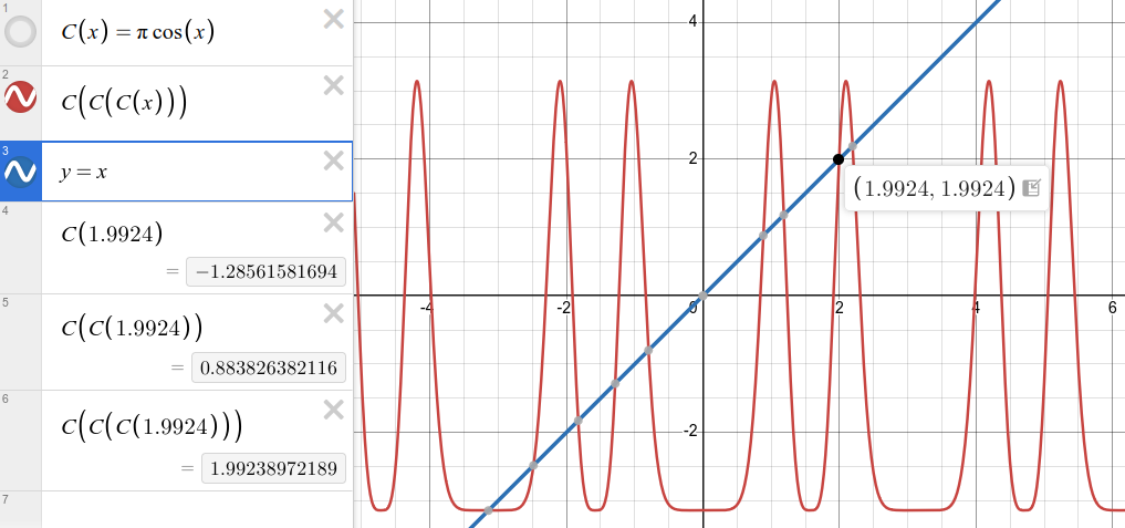
It turns out that there are several intersections. But be careful! Some of those are actually \(1\) and \(2\)-cycles. Checking \(x_0=1.9924\), we see that it indeed cycles from: \[x_0 = 1.9924 \] \[x_1 = -1.2856 \] \[x_2 = 0.8838 \] \[x_3 = 1.9924 \] It is true that the value \(x_0=1.9924\) is not exact, but we can at least see graphically that the point exists, it is part of a \(3\)-cycle, and it is very close to \(1.9924\).
Chaotic Orbit
Some dynamical systems exhibit a phenomenon known as chaos. Chaos refers to a system that is deterministic but which exhibits sensitive dependence on initial conditions.
Determinism is the concept that given initial conditions and the set of laws to be followed, all future states of a system can be determined exactly. That is, a deterministic system is theoretically a predictable system.
Sensitive dependence on initial conditions means that even extremely small variations in inital conditions can lead to completely different behaviors or predictions. Recall Poincaré in Science and Reason who concluded that because "we could still only know the initial situation approximately", "prediction becomes impossible". It is not that we cannot measure, and it is not that we cannot predict, but that to make perfect predictions would require both perfect models and perfect data, which do not exist. (Quantum mechanics is also sitting over there waiting to say something!)
The graph below depicts two orbits in the same dynamical system, for nearly identical initial values \(x_0\).
\(x_0 = 8.00001\)
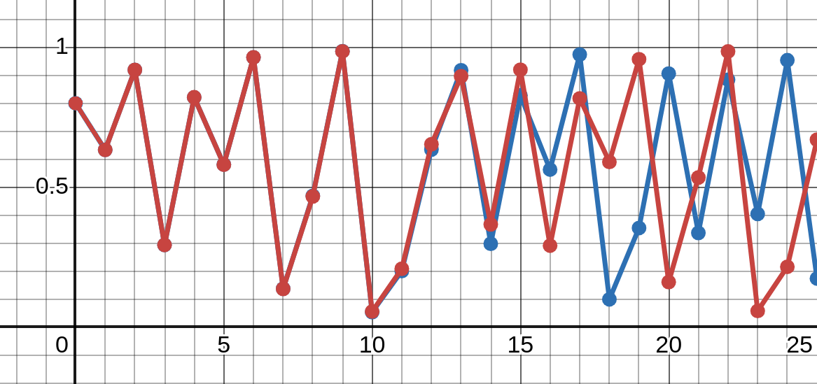
The orbits are indistinguishable for ten iterations, but then separate into two completely different behaviors which will never meet again.
The concept of chaos has profound implications for our understanding, building, and deploying of data models.